How to Evaluate Optical Performance in Rigid Endoscopes

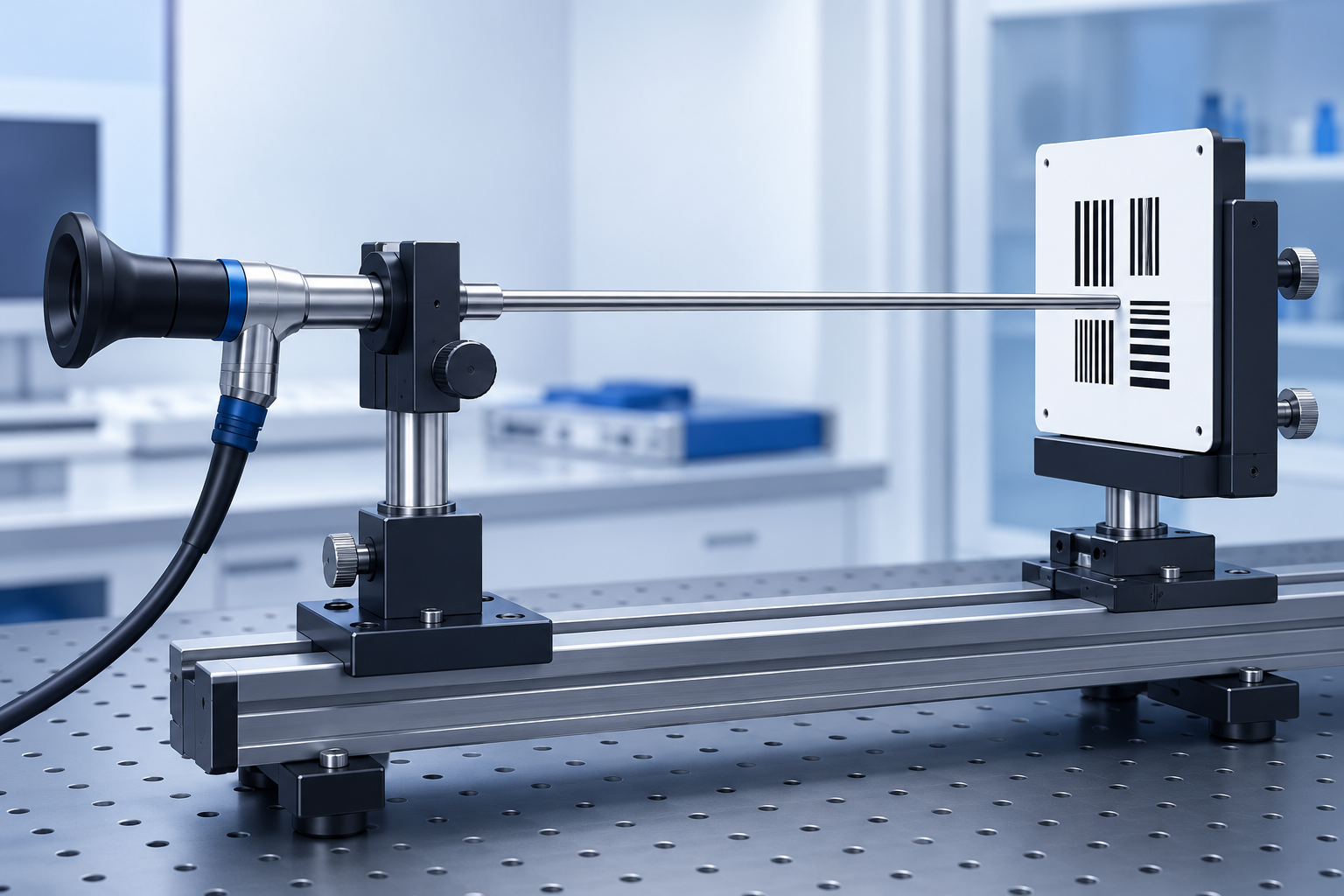
An endoscope demonstration can be visually convincing yet leave an optical engineer with very little comparable evidence. Automatic exposure can conceal a throughput difference; sharpening can accentuate edges; a coupler can show only the strongest part of the field. The displayed image contains contributions from every component between the object and the observer.

A useful evaluation separates the rigid scope’s optical contribution from the behaviour of the assembled imaging system. It combines measurements of geometry, spatial detail, light transfer and focus with a record of the test configuration. One excellent centre-resolution result cannot establish uniform optical quality. The framework below is an engineering approach to planning that evaluation, not a set of universal acceptance limits or a report of product performance.

1. Define what you are actually evaluating

Scope-only optical characterization asks how the scope forms and transfers an image under defined conditions. Relevant properties include field and direction of view, spatial response, centre-to-edge consistency, distortion, focus, spectral transmission and unwanted light. Mechanical alignment matters because the objective, relay optics and eyepiece must operate as an assembly.

“Scope-only” still requires measurement equipment. A camera used as a measuring instrument must have adequate sampling and a characterized response; its coupling optics cannot silently limit the result. Name the measurement boundary explicitly. A result acquired through an uncharacterized camera attachment is evidence about that combination, even if the report is headed “scope resolution.”

System-level image evaluation includes the coupler, camera head and sensor, processor, electronic sharpening, exposure, gain, white balance, illumination, display and any capture compression. It answers the integration question: what image does this particular combination deliver? Both levels are useful, but their conclusions need separate labels.

1. Target / objectDefined geometry and illumination
2. RIGID OPTICAL SCOPEScope characterization
3. Coupler / camera headOptical interface
4. Image sensorSampling and detection
5. ProcessorImage processing
6. DisplayPresentation to the observer

A 4K camera or monitor cannot recover optical information already lost in the scope. A 3840 × 2160 output describes the image raster, not a measured optical resolving capability. “4K-ready” is meaningful only as a system-matching proposition supported by the tested scope, coupler, sensor sampling and processing configuration. Ask for that evidence rather than treating the label as a resolution unit.

2. Build a controlled test configuration

A comparison begins with a configuration record, not a favourite demonstration image. Identify the scope and revision, target, working-distance reference, mounting orientation, camera and coupler, light source and acquisition settings. Photograph the setup and save settings with the original files. Establish the focus rule before collecting results so that an operator cannot unintentionally favour one sample.

Variables to control during comparative scope evaluation

Variable	Why it matters	Typical control approach
Working distance	Changes object scale and focus demand	Fix and document the distance and reference plane
Scope-to-target alignment	Tilt or offset can create apparent field differences	Use repeatable mounts; record viewing-axis orientation
Camera / coupler	Changes sampling, image scale and captured field	Keep identifiers, optics and sensor mode fixed
Focus setting	Local optimization can hide field-dependent defocus	Define the focus criterion and permitted adjustments
Exposure	Alters signal level and clipping	Lock where possible; document actual values
Gain	Changes noise and displayed contrast	Fix gain; record any unavoidable automatic behaviour
Sharpening / image processing	Changes edge appearance and tonal response	Disable enhancement where feasible, or lock and document it
Illumination	Changes target radiance and spatial distribution	Stabilize source, coupling, spectrum and setting
Target	Texture, contrast and flatness affect the measurement	Identify a suitable target and check its condition
Capture method	Resizing and compression can alter fine detail	Preserve native captures and processing history

If automatic control cannot be disabled, record its response and narrow the conclusion accordingly. Identical menu settings do not prove identical exposures after exchanging scopes. White balance, noise reduction, gamma and image-processing mode also belong in the record. Keep display adjustment separate from recorded pixel data.

Repeat selected measurements after removing and remounting the same scope. This distinguishes setup repeatability from sample variation before a small difference becomes a procurement ranking. A bench reference can help reveal drift, but it also needs a stability record. Record uncertainty, exclusions and failed captures alongside the accepted results; do not replace them with a single best frame.

3. Field geometry comes before image sharpness

Field of view describes the angular scene coverage; direction of view describes the orientation of observation relative to the scope’s longitudinal axis. The familiar 0° and 30° labels concern direction, not field size. Working distance connects the observed angular field to the object area represented. A camera crop or a different coupler can change the displayed coverage without changing the scope itself.

ISO 8600-3:2019 2 addresses measurement of field and direction of view. Its public abstract distinguishes methods using different distance references. Declare the reference geometry and follow the applicable standard or validated internal method; a screen estimate is not a substitute.

Distortion concerns the mapping between object and image geometry. It changes local magnification across the field and can influence spatial perception; it is a separate attribute from blur or resolving power. Low distortion does not establish high resolution. The distinction is explained in the optical-design reference 5. A straight-looking processed grid also needs its correction settings recorded.

For comparative work, retain a distortion map or field-dependent description rather than only one extreme value. Check target alignment before attributing asymmetry to the scope. Compare the uncropped field where accessible, then document the portion delivered by the intended camera. Geometry establishes where subsequent resolution and illumination observations actually belong.

4. Measure resolution, contrast and field consistency

Limiting resolution asks how fine a pattern can still be distinguished under the selected criterion. Contrast at lower spatial frequencies asks how strongly coarser structures remain differentiated. Spatial-frequency response describes behaviour across a range of detail sizes. These answer different engineering questions: identifying a fine pattern at low contrast does not describe how the instrument renders broader structure.

ISO 8600-5:2020 3 applies to optical resolution evaluation of medical rigid endoscopes with optics; its stated scope excludes endoscopes with fibre-optic or opto-electronic imaging systems. This is an imaging-path distinction, not an exclusion of a rigid optical scope merely because it uses fibres for illumination. The official abstract identifies three characteristics: A, limiting resolution; B, low-spatial-frequency resolution associated with image sharpness or contrast; and C, spatial-frequency response. This article does not reproduce the standard’s test procedures.

MTF describes contrast transfer as a function of spatial frequency. It gives context that one limiting-resolution value cannot provide. ISO 8600-5 defines specific optical-resolution characteristics. Its Characteristic C concerns spatial-frequency response; it should not be assumed equivalent to a complete MTF measurement. A useful curve identifies the frequency units, object or image reference, field position and focus condition. The general MTF framework is introduced in reference 4.

Keep measured curves separate from optical-design predictions. Include acquisition response in the interpretation: sampling, sharpening and nonlinear tonal processing can change the apparent response. A more pronounced edge after sharpening is not proof that the scope transmitted additional information. Inspect the original capture and processing settings before using the enhanced image to support a resolution claim.

A strong on-axis result can coexist with weak peripheral contrast. Decentration, tilt, relay-stack alignment error or residual aberration are possible contributors, but so are target and camera alignment. Compare centre, mid-field and representative near-edge positions, including symmetry. Preserve the field orientation when recording results; averaging opposite sides too early can conceal a repeatable imbalance.

CMMMMEEEE

• C — Centre
  On-axis reference
• M — Mid-field
  Up, down, left and right
• E — Near-edge
  Representative peripheral positions

A fixed-focus field map and a map refocused at each position answer different questions. The first describes simultaneous field performance at one setting; the second helps investigate local best performance and field-dependent focus. Retain both labels when using both approaches. Compare pattern orientations as well as locations where the method calls for it, and avoid diagnosing an internal element from a screenshot alone.

What image behaviour may be telling you

Possible contributors — not a fault diagnosis by image appearance alone. These are engineering investigation prompts, not standard acceptance criteria.

Observed behaviour	Possible optical / mechanical contributors	What to investigate
Good centre, weak edge	Field aberration, tilt, decentration, relay alignment	Field map, focus rule, target and coupler alignment
Left-right asymmetry	Decentration or mechanical alignment; setup error	Repeat mounting; track orientation and field position
Reduced contrast with apparently sharp edges	Sharpening, tonal processing or stray-light interaction	Native capture, enhancement settings and bright-source response
Veiling haze	Scatter, contamination or internal reflections	Accessible surface condition and controlled illumination
Ghost image	Surface reflections, coating behaviour or internal geometry	Repeatable source position, interfaces and spectral band
Uneven field brightness	Illumination coupling, vignetting or alignment	Uniform target, source delivery and camera shading correction

5. Evaluate transmission, illumination and unwanted light

Transmission requires an input/output measurement boundary and a defined spectral band. Separate the scope’s imaging path from the illumination path that delivers light to the object. For a spectral measurement, document detector response, collection geometry and reference measurement. A coating datasheet or a value for one glass element cannot stand in for the assembled scope.

Apparent image brightness is a system-level observation. A transmission comparison requires controlled illumination, exposure, gain, spectral response and processing, with a defined measurement reference. Automatic exposure may make two unequal signals look similarly bright. Conversely, a different scene or light-guide coupling may make the same scope appear brighter. Compare recorded signal under controlled conditions before making a throughput judgment.

For field uniformity, use a characterized uniform scene and examine the spatial pattern before normalization. Investigate source delivery, vignetting, optical alignment and camera shading correction separately. A corrected image can be relevant to system use, while the uncorrected record is more useful for locating the contribution. Keep both when available.

Stray light is unwanted light reaching the imaging path. It may produce broad veiling glare that reduces contrast or a more discrete reflection artefact, a ghost. Surface contamination, scatter, coatings and internal reflections are possible contributors. Move a controlled bright source through documented positions while monitoring clipping and exposure. Check permitted external cleaning and interface conditions before considering an internal cause; this is not a direction to disassemble a medical device.

Final colour reproduction combines illumination spectrum, scope spectral transmission, camera spectral response, white balance, processing and display behaviour. A scope transmission spectrum describes only one contribution. Evaluate colour with a defined target and capture/display conditions, and report it as a system result unless the experiment specifically isolates the component.

6. Focus, chromatic behaviour and fluorescence-specific considerations

Define best focus using a stated criterion and record where it occurs. Then vary object distance under controlled conditions to examine the range over which the required detail remains acceptable. “Depth of field” without an acceptance criterion leaves too much room for observer preference. Record whether the coupler is refocused and whether image scale changes during the sequence.

Glass dispersion makes refractive power wavelength-dependent, so focus and field behaviour can change with spectral band. Axial chromatic behaviour shifts the focus position; lateral chromatic behaviour shifts image position or magnification with wavelength. General optical context is provided in references 6 and 7. Coloured edges alone cannot identify which component is responsible.

Additional evaluation for fluorescence scopes

Evaluate visible-to-NIR parfocality by characterizing axial focus shift between the two spectral regions. A parfocal design aims to minimise the shift and the refocusing needed when switching modes. Its amount and direction depend on the optical design, glass selection and chromatic correction. Characterize both bands with a documented target, band definition, focus criterion and acquisition configuration. Report residual shift or the corresponding performance at a shared focus setting; avoid promises of zero shift or no refocusing without supporting measurements.

When investigating a scope, separate its chromatic contribution from that of the coupler and camera optics. When evaluating an assembled system, also measure the user-facing consequence of switching modes. A scope-level result cannot establish parfocal behaviour for every camera attachment.

The additional investigation plan can include:

• Visible and NIR spectral transmission through the defined imaging path.
• Visible/NIR focus shift and field performance at a common focus setting.
• Spectral leakage and rejection of excitation light in the complete filtering arrangement.
• NIR stray light, ghosting and signal uniformity using a suitable stable reference.
• Channel registration across the field and working range where applicable to the imaging architecture, particularly when separately acquired visible and NIR images are combined.

Fluorescence detection requires separation of excitation from emission; reference 8 explains the optical-filter principle. The displayed brightness also reflects the excitation source, sample response, scope NIR throughput, filters, detector sensitivity, exposure, gain, processing and display mapping. Bright green rendering alone cannot isolate scope performance. Document the reference material and processing before comparing modes or samples. The related ICG fluorescence article develops the imaging context further.

7. Beyond the initial bench test: alignment, reprocessing and sample consistency

An initial optical pass describes the sample in its measured condition. Where lifecycle performance is part of the requirement, reassess critical optical characteristics after the intended validated reprocessing exposure. Compare with baseline measurements using the same method and a stable reference. Cycle counts, temperatures and chemicals belong to the device’s validated instructions and verification plan, not a generic article.

The investigation can consider distal-window condition, seal integrity, contamination, thermal effects, mechanical stress and alignment of the relay train, eyepiece and interface. A change in optical-axis position or field symmetry warrants controlled follow-up. A shifted measurement is not sufficient to attribute failure to a seal, adhesive or individual lens. Record handling and mounting history before assigning a cause.

For supply consistency, request individually identified samples and their revision or lot context. Repeatability on one unit and variation across units are different questions. Preserve individual field maps and outliers as well as summary statistics. A sample plan selected for verification or production control needs its own rationale; a few selected demonstration units cannot establish future production consistency.

Field consistency, geometric representation, flare, focus stability and illumination distribution can affect what a user sees and how the imaging system is handled. Optical bench measurements characterize device behaviour; they do not, by themselves, demonstrate clinical benefit. Claims about outcomes, complications or diagnostic performance require separate evidence.

8. From measurements to an engineering decision

The useful supplier question is more specific than “What is the resolution?” Ask which configuration and working distance were tested; whether the result isolates the scope; which field positions and processing settings were used; and what acceptance specification applied. Request the method revision, uncertainty and sample identity with the data. For fluorescence integration, include visible/NIR focus-shift characterization and the tested channel arrangement.

A complete discussion also asks whether performance was checked after validated reprocessing and how unit-to-unit consistency is monitored. Agree the decision before selecting a preferred sample: design investigation, incoming inspection and system integration do not necessarily use the same evidence package. The matrix below organizes that discussion; it does not set pass limits.

A practical evaluation framework

Property	Scope-only evaluation	System-level influence	Common interpretation risk
Field of view	Angular coverage with declared reference	Coupler and sensor crop	Displayed crop mistaken for scope field
Direction of view	Observation orientation relative to shaft	Mounting and image rotation	Direction mistaken for field size
Resolution	Spatial detail under a defined method	Sampling and enhancement	Pixel count treated as optical resolution
Field consistency	Location and symmetry maps	Coupler or sensor tilt	Centre result generalized to whole field
Distortion	Geometric mapping	Digital correction and crop	Straight lines treated as sharpness evidence
Transmission	Defined spectral input/output comparison	Source and detector response	Brightness treated as throughput
Brightness	Not isolated by display appearance	Exposure, gain and tone mapping	Automatic compensation overlooked
Colour	Spectral transmission contribution	Source, sensor, balance and display	Whole-system accuracy assigned to scope
Stray light	Controlled unwanted-light response	Interfaces and processing	A screenshot treated as root cause
Focus	Criterion and distance-dependent response	Coupler adjustment and sampling	Different focus rules compared
Visible/NIR parfocality	Band-dependent axial focus behaviour	Camera optics and channel arrangement	One combination generalized to all systems
Illumination uniformity	Defined delivery or imaging-path contribution	Coupling, scene and shading correction	Combined field pattern assigned to one part

Key takeaways

1. Identify whether the measurement characterizes the scope or the complete imaging chain.
2. Control and record the configuration before comparing samples.
3. Evaluate centre, field positions and symmetry together.
4. Treat displayed brightness, colour and fluorescence as system observations unless their contributions are isolated.
5. Interpret geometry, spatial response, transmission, unwanted light, focus and consistency together rather than reducing quality to one number.

References

Official standard records and optical-engineering references below were consulted on 6 October 2026. The proposed control plan, diagnostic prompts and comparison matrix are engineering interpretations, not normative procedures.

1. ISO 8600-1:2025. Endoscopes — Medical endoscopes and endotherapy devices — Part 1: General requirements. Official ISO record. General terminology and requirements context; this article does not provide a conformity assessment.
2. ISO 8600-3:2019. Endoscopes — Medical endoscopes and endotherapy devices — Part 3: Determination of field of view and direction of view of endoscopes with optics. Official ISO record.
3. ISO 8600-5:2020. Optics and photonics — Medical endoscopes and endotherapy devices — Part 5: Determination of optical resolution of rigid endoscopes with optics. Official ISO record.
4. Edmund Optics. Introduction to Modulation Transfer Function. Optical-engineering reference.
5. Edmund Optics. Distortion. Imaging Resource Guide.
6. Edmund Optics. Aberrations. Imaging Resource Guide.
7. Edmund Optics. Wavelength Effects on Performance. Imaging Resource Guide.
8. Edmund Optics. Introduction to Fluorescence Filters: Principles, Selection, and Applications. Optical-filter reference.

Standards note. ISO 8600-3:2019 and ISO 8600-5:2020 remain the current published editions referenced here at the time of writing; revisions are under development. Formal verification should use the current published edition and the manufacturer’s validated test procedures. This article is not a substitute for either.